LIGO/Virgo maps, I/O and resampling
On this example we’ll use LIGO/Virgo skymaps as an excuse to see how to open/write a map to/from disc, how create a multi-resolution maps out of a single-resolution map, and how to resample an already multi-resolution map.
Reading a map
Both single and mult-resolution maps are stored in FITS files. While you can download a map and then provide the local path, you can also use the URL directly, e.g.
[1]:
from mhealpy import HealpixMap
# GW170817!
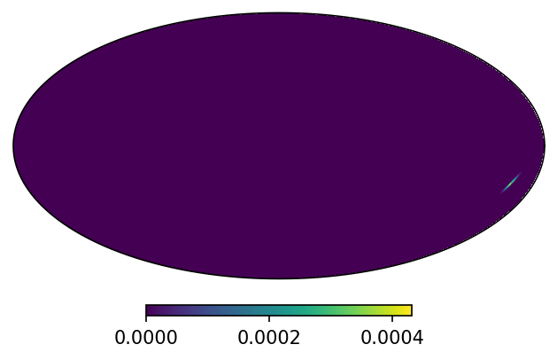
m = HealpixMap.read_map("https://dcc.ligo.org/public/0157/P1800381/007/GW170817_skymap.fits.gz", density = False)
m.plot();
[2]:
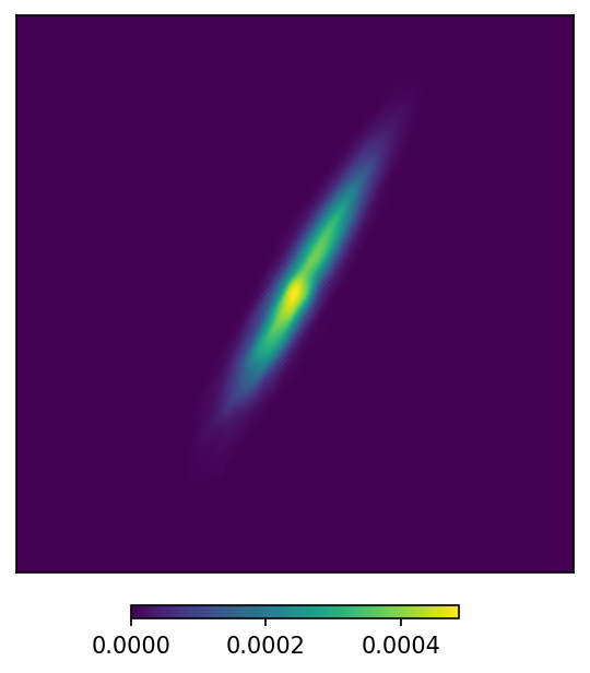
# Zoom in around the maximum

import numpy as np

theta_max,phi_max = m.pix2ang(np.argmax(m))

lonra = np.rad2deg(phi_max) + np.array([-10,10])
latra = (90-np.rad2deg(theta_max)) + np.array([-10,10])

m.plot(ax = 'cartview', ax_kw = {'latra': latra, 'lonra': lonra});
Single to multi-resolution
The map we just opened is a single resolution map. Since this is a well-localized event the full sky is sampled at a relatively high resolution.
[3]:
print("Is multi-resolution? {}".format(True if m.is_moc else False))
print("nside: {}".format(m.nside))
print("# of pixels: {}".format(m.npix))
Is multi-resolution? False
nside: 1024
# of pixels: 12582912
We can create a multi-resolution map by setting the condition that the probability assigned to any given pixel is at most the maximum value of the current single-resolution map. This mitigates the loss of information and results in a fair sampling for all locations.
[4]:
mm = m.to_moc(max_value = max(m))
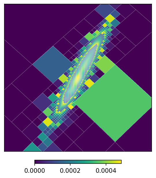
mm.plot(ax = 'cartview', ax_kw = {'latra': latra, 'lonra': lonra});

While this plot looks pretty much the same as before, we reduced the number of pixels by 3 orders to magnitude.
[5]:
print("Is multi-resolution? {}".format(True if mm.is_moc else False))
print("nside: {}".format(mm.nside))
print("# of pixels: {}".format(mm.npix))
Is multi-resolution? True
nside: 1024
# of pixels: 4026
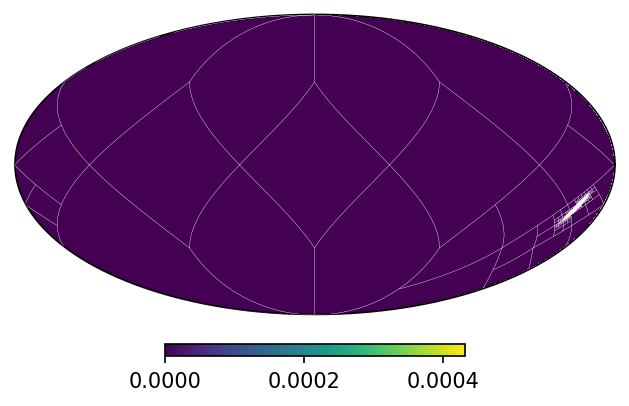
We can see the way this works more clearly by superimposing the grid
[6]:
import matplotlib.pyplot as plt

mm.plot()
mm.plot_grid(plt.gca(), linewidth = .1, color = 'white');
[7]:
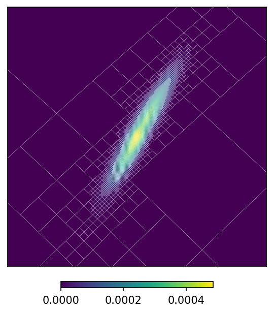
# Zoom in
mm.plot(ax = 'cartview', ax_kw = {'latra': latra, 'lonra': lonra})
mm.plot_grid(plt.gca(), linewidth = .1, color = 'white');
By default the equivalent to the rasterized map is plotted. That is, the previous plot is proportional to the probability density distribution, rather than the integrated probability on each pixel. You can changed this behaviour using the rasterize option.
[8]:
mm.plot(ax = 'cartview', ax_kw = {'latra': latra, 'lonra': lonra}, rasterize = False)
mm.plot_grid(plt.gca(), linewidth = .1, color = 'white');
The function to_moc() is a convenience routine derived from adaptive_moc_mesh(). The same is true for moc_histogram() and moc_from_pixels(). In the more general adaptive_moc_mesh() the user provides an arbitrary function that decides, recusively, whether a pixel must be split into child pixels of higher order or remain as a single pixel.
Resampling multi-resolution maps
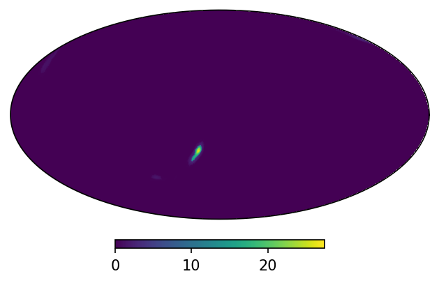
For new gravitational wave events LIGO/Virgo also provides multi-resolution maps straight out the box, e.g.
[9]:
from mhealpy import HealpixMap

m = HealpixMap.read_map("https://gracedb.ligo.org/api/superevents/S200219ac/files/LALInference.multiorder.fits,0", density = False)

print("Is multi-resolution? {}".format(True if m.is_moc else False))
print("nside: {}".format(m.nside))
print("# of pixels: {}".format(m.npix))

m.plot();
Is multi-resolution? True
nside: 512
# of pixels: 16896
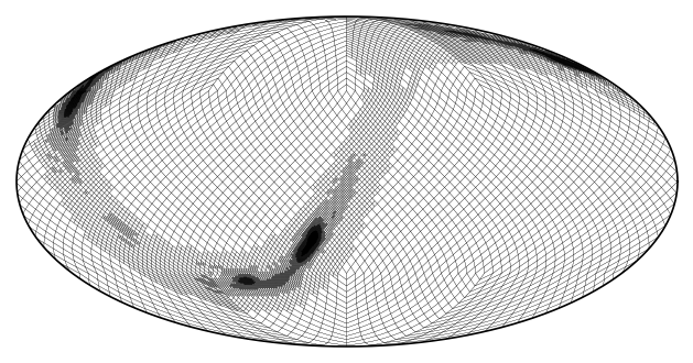
The grid though corresponds to the adaptive mesh used to generate the sky localization:
[10]:
m.plot_grid(linewidth = .1);
We can resample it the same way we did for the single-resolution map:
[11]:
mm = m.to_moc(max(m))

print("Is multi-resolution? {}".format(True if mm.is_moc else False))
print("nside: {}".format(mm.nside))
print("# of pixels: {}".format(mm.npix))

mm.plot_grid(linewidth = .1);
Is multi-resolution? True
nside: 512
# of pixels: 5616
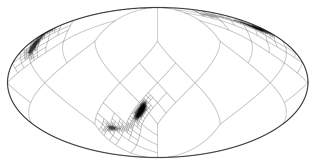
While only a modest improvement in this case, resampling can be useful when the map is the product of maps from multiple sources. As seen in the quick start tutorial, in order to assure there is no information loss, the grid resulting from an operation is the union of the grid of its operands. This can result in high resolution in regions where it is no longer needed.
Writing a map to disc
We can now save this resampled map to disc.
[12]:
mm.write_map("S200219ac_LALInference_resampled.multiorder.fits")
The format is compliant with the the IVOA MOC recommendation. The map is saved into the second (0-th indexed) HDU as an extension table, each pixel specified explicitely by its UNIQ number:
[13]:
from astropy.io import fits

f = fits.open("S200219ac_LALInference_resampled.multiorder.fits")

f[1].header
[13]:
XTENSION= 'BINTABLE'           / binary table extension
BITPIX  =                    8 / array data type
NAXIS   =                    2 / number of array dimensions
NAXIS1  =                   16 / length of dimension 1
NAXIS2  =                 5616 / length of dimension 2
PCOUNT  =                    0 / number of group parameters
GCOUNT  =                    1 / number of groups
TFIELDS =                    2 / number of table fields
TTYPE1  = 'UNIQ    '
TFORM1  = 'K       '
TTYPE2  = 'CONTENTS'
TFORM2  = 'D       '
PIXTYPE = 'HEALPIX '           / HEALPIX pixelisation
ORDERING= 'NUNIQ   '           / Pixel ordering scheme: RING, NESTED, or NUNIQ
COORDSYS= 'C       '           / Celestial (C), Galactic (G) or Ecliptic (E)
NSIDE   =                  512 / Resolution parameter of HEALPIX
INDXSCHM= 'EXPLICIT'           / Indexing: IMPLICIT or EXPLICIT
MOCORDER=                    9 / Best resolution order